FOUR-DIMENSIONAL INFORMATIONAL SETS IN A PROBLEM OF AIRCRAFT TRACKING

1. Krasovskii N.N., Subbotin A.I. Positional Differential Games. Nauka, Moscow, 1974 (in Russian).
2. Kurzhanski A.B. The Control and Observation in Uncertainty Conditions. Moscow, Nauka, 1977 (in Russian).
3. Chernous'ko F.L., Melikyan A.A. Game Problems of Control and Search. Moscow, Nauka, 1978 (in Russian).
4. Milanese M., and Norton J.P., Eds. Bounding Approaches to System Identification, Plenum Press, London, UK, New York, 1996, USA.
5. Maksarov D. and Norton J.P. State bounding with minimal volume ellipsoids. Proceedings of UKACC International Conference on CONTROL'96, 2-5 September 1996, IEE, UK. Publication No.427, pp.1297-1302.
6. Isaacs R. Differential games. Wiley Inc., New-York-London-Sydney, 1965.
7. Berdyshev Yu.I. Time-optimal control synthesis for a fourth-order nonlinear system. Prikl. Mat. Mekh. 39(1975), No.6, pp.985-994 (in Russian).
8. Kumkov S.I., Patsko V.S. Control of Informational Sets in a Pursuit Problem. Annals of the International Society of Dynamic Games, New Trends in Dynamic Games and Applications. G.J.Olsder, Ed. Birkhauser, Boston, 1995, pp.191-206.
9. Emelyanov D.D. Optimal impulse control of the informational set in a homing problem with incomplete information. Avtomatika i Telemekhanika, No 1, 1998, pp.35-45 (in Russian).
10. Patsko V.S., Pyatko S.G., Kumkov S. I., Fedotov A.A. Informational sets in problems of aircraft tracking. Published by the Academy of Civil Aviation, St.-Petersburg, and the Institute of Mathematics and Mechanics of Ural Branch, Russ. Acad. Sci., Ekaterinburg, 1999.

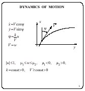
A model problem of aircraft tracking is considered. Aircraft motion is described in the horizontal plane x, y by a system of differential equations of the fourth order. Here, x, y are geometrical coordinates of the aircraft position; is the heading; V is the velocity value; the constant k is the maximal value of the lateral acceleration; u, w are unknown controls, which obey geometric constraints.

In general, a relation, that determines the velocity dynamics, can be more complicated than the fourth equation of the system. Such a relation can depend on many parameters and can not be known exactly. Refusing a complicated description, we use the equation and interpret parameters as constraints on possible values of the longitudinal acceleration .

The system is often used for description of motion of an aircraft, a car, and other objects with similar dynamics.

Current information about aircraft motion is represented in a form of measurements of its position in the plane at discrete time instants. The geometric constraint on the measurement error is given. The heading and velocity V are not measured. An approach based on a construction of the informational sets is applied for solving the problem of aircraft tracking.

As an informational set we mean a totality of all phase states of the system consistent with all measurements received up to the current instant.

Theoretical questions joined with informational sets in different problems were investigated in works of N.N.Krasovskii, A.B.Kurzhanskii, A.I.Subbotin, F.L.Chernous'ko and their colleagues. But a few works concern a construction of the informational sets in concrete problems. It is stipulated by the fact that in concrete cases the informational sets can have very complicated structure.

In the problem considered, the informational sets are built in a four-dimensional space and are not convex. More than that, they can be disconnected.

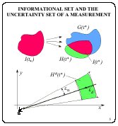
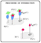
Explain now the general scheme of construction of the informational sets. Let an informational set be constructed for the instant , and suppose that the next measurement comes at the instant . Using the dynamics description, the forecast set is built. This is an attainability set of the controlled system at the instant with the set as the initial one. The uncertainty set is put in correspondence to the measurement obtained at the instant . This is a totality of all phase states consistent with the measurement and the given constraints on the measurement error. The informational set is constructed as the intersection of the sets and . In the problem discussed, measurements of an aircraft position in the horizontal plane are obtained, for example, from a radar. The measurement error is stipulated by errors in the direction and distance, and the corresponding set of positions in the horizontal plane appears. The set , being a set in the four-dimensional phase space, is cylindrical in coordinates , V and has the set as a projection in the plane x, y. Further, the sets are supposed to be convex.

Note two special properties of the equation system: 1) the third and fourth equations do not depend on the first and second ones, 2) the phase variables x, y are not present in the right-hand side of the first and second equations.

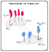
It allows to construct the informational sets in the following way. A projection of the informational set into the plane , V is considered. A set is put in correspondence to each point of the set . Each set is a section of the set by a plane {=const, V=const} and is described by its projection into the plane x, y. As the first operation when building the full forecast set, we compute the forecast set taking the set as the initial set.

Several motions from the set come to each point , of the set . Along each motion the corresponding set is transferred, and the transferred sets are further united. In such a way, we obtain the set . Having implemented this operation for all pairs , , we obtain the forecast set , which is represented in the same form as the set .

The main difficulty is in the fact that the sets are not convex. We consciously make some roughening when substitute the set by its convex envelope .

So, instead of the true forecast set , we obtain its upper estimate represented by a nonconvex set and a totality of convex sets .

The informational set is an intersection of the forecast set and the uncertainty set . The form of representation of the set and the cylindrical property of the set in the coordinates , V permits us to implement this intersection in a rather simple way. Namely, we intersect each set with the set . These sets are convex and lie in the plane x, y. Nonempty results of the intersection compose the informational set .

Underline once more that under exact construction of the informational sets their sections are not convex. In our constructions, the sets are convex and give upper approximations of the true sets . We apply the operation of convexification from the initial time instant t₀.

In practical building the informational sets, the set is given by a grid, and the sets , corresponding to each node , V of the grid, are convex polygons.

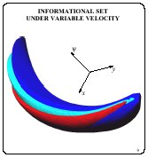
Choose in the set all nodes with the same value of the velocity V and gather a totality of corresponding sets . This totality represented for different values of the coordinate composes a three-dimensional set. If the grid in is sufficiently dense, then obtained informational set practically coincides with the section of the set I(t) for chosen value of V. The film shows three such sets for three different values of V. Their "banana" form is typical for the problem under discussion.

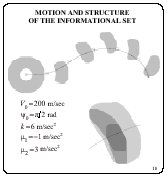
Elaborated program for the informational set construction allows to implement calculations in a real-time tempo. The simulation results are shown for the time interval 120 sec. Projections of the informational set are shown in the plane x, y. The initial uncertainty in was given from 0 to , and in V it was from 100 m/sec to 500 m/sec.

The large uncertainty in had stipulated the ring form of the forecast set in the initial time interval. The thing solid line marks the trajectory of the true motion. Measurements came with the time step of 20 sec.

In intervals among the measurements appeared, the informational set grows; when the next measurement comes, the set fast decreases.

The informational set at the instant 53 sec is shown in detail. Here, the whole projection is marked in light gray, the layer corresponding to the velocity value of 277.8 m/sec is shadowed in middle gray. Inside, one section of the informational set is marked in dark gray for the value =1.173 rad. All these section gathered for all admissible compose the layer (middle gray) for the given V.

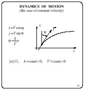
The case, when the velocity is known in advance and constant in time, is interesting itself. Here, the motion dynamics is described by a system of three differential equations. Respectively, the informational set is built in the three-dimensional space.

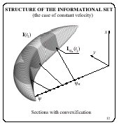
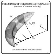
In the case when the velocity is known in advance and constant in time, the informational set is composed of the sections (layers) which correspond to each node of the grid in . Each section is a convex polygon because of the way of its building (Film 12). Without convexification, the sections could be non-convex as presented in the Film 13.

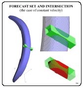
For some instant, the forecast set is shown in blue. The uncertainty set of the measurement appeared colored in green. The uncertainty set is cylindrical in the coordinate . The area of the intersection and its result are shown in a large scale. The obtained informational set is marked in red.

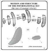
A fragment of the informational set motion in the interval of 32 sec is shown in a projection in the plane x, y. In this interval, there are two measurements with the uncertainty sets in the form of a parallelogram (a) and a rectangle (b). The crosses mark positions of the true point. In the informational set, the layers are shadowed which located in mostly close to its corresponding true values.

The three-dimensional structures are shown around the instant (a): before (the forecast set) and after (the informational set itself) taking into account the measurement at this instant. It is seen that the informational set is evidently improved in the non-observable coordinate : the layers corresponding to non-admissible values of are eliminated - they give empty intersections with the uncertainty set of the measurement.

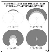
Remind, that the applied procedure of convexification leads to an error in the construction of the informational set. To estimate this error, we compare the constructed forecast sets with exact attainability sets calculated under special conditions. Suppose that the initial position of an aircraft and the initial heading are exactly known, and the value of the velocity is also known and constant. For this case, the exact formulae are known, which describe the frontier of the attainability set in the projection in the plane x, y. The comparison is illustrated by the attainability sets (contoured by the solid line) for four time instants. The instants correspond to change of the heading in . The forecast sets calculated by our algorithms are shadowed in gray. The arrows mark the initial heading of the velocity vector, and the circles represent trajectories with the extreme controls u=-1 and u=1. Each figure has its own scale. It is seen that the outer frontiers of the forecast sets and the attainability sets practically coincide, but their inner frontiers are different. (For calculation of the exact attainability sets, the formulae were used from the works of Yu.I.Berdyshev.)

Underline that the frontier of the exact attainability set can be calculated only for a point-wise initial set. But usually, in problems with incomplete information, it is necessary to build the forecast set having the initial set of a rather arbitrary form. Moreover, the construction has to be implemented in a three-dimensional space if the value of the velocity is known, and in a four-dimensional space if this value is unknown. The approach elaborated for building the forecast set does not give the exact result, but provides an upper approximation of the true sets and is rather simple in numerical realization.